Environmental factors affecting AFL outcomes – the weather

As part of my previous piece that began to explore elements of home ground advantage (HGA), I identified that in order to be able to isolate the effects of HGA, one would need to first account for player performance, team performance and other environmental factors.

A model to predict the outcome of a sporting match

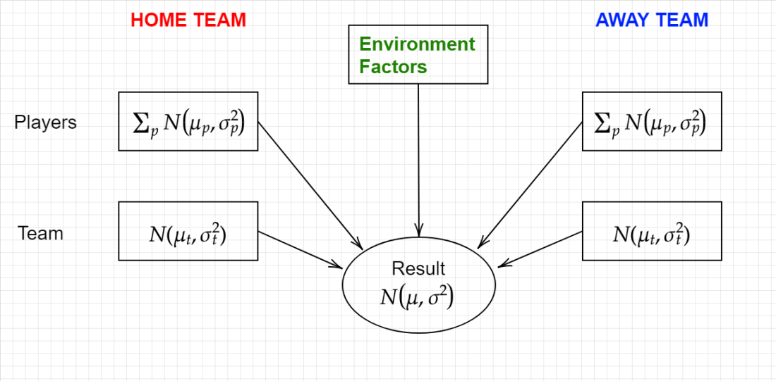
As discussed in the previous piece, the environmental factors consist of of many measurable and immeasurable modifiers that affect the outcome of a game. This could include home ground advantage, the weather, if a team is coming off a short break, if a team has traveled a lot lately, if players are carrying injuries, if there’s a player milestone, if it’s a “rivalry” game, and the list goes on. Some of these are easier to look at than others. In time I hope to investigate and, if necessary, account for all of these factors.

In this piece, I’m going to focus on the weather conditions and how they affect the outcome. Like my previous piece, there are more questions than answers at the moment. Nevertheless, I hope you find this thought-provoking!

Wet Weather Football

Playing in the wet is a different game altogether. The physics of the game changes. The ball is slippery; making slick handballs too slick, contested marks rare and ground ball pickups difficult. The players are slippery; tackles don’t stick as well. The slippery ground however makes the ball bounce a little straighter so there are benefits to exploit, but I digress. It’s easy to argue that wet weather affects the game, but how can we measure it?

“Now over to Tony Greig at the weather wall”

The lads that manage fitzRoy (a magnificent package for those interested in a leg-up start in probing AFL stats) include some BoM rainfall data for each match in the 2017 season; which seems like a good place to start. From BoM I scraped historical rainfall data from the nearest weather stations to each AFL ground and attached the game day’s rainfall to each game from 2011 onwards. There were plenty of gaps in the data, from 1563 games I ended up with 953 records. The standard stereotype of wet weather football is low scores. Below I present a set of histograms of the total points scored in matches with different daily rainfalls.

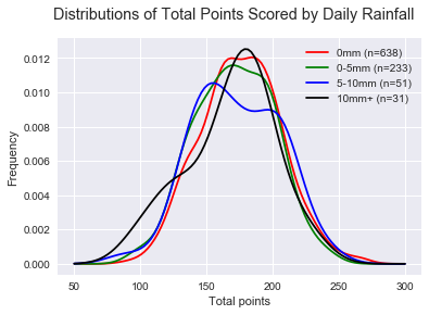
Wow! Either rain has little effect on the total points scored, or these daily rainfall figures do not represent the conditions at the football ground during the match.

In Round 5, 2015, the Gold Coast local weather station recorded a daily rainfall aggregate of 132mm after 9am. By 4:35pm when the Suns took on the Lions, the ground was seemingly dry and there was no report of wet/slippery weather and scoring certainly wasn’t affected. These types of anomalies (I’m sure there are many) make the daily rainfall near the ground a poor measure of the actual effect of the rain on the game.

While this annoyed me a bit; quite a bit of time was spent scraping and organising the rainfall data, it did illuminate a possible next step. As mentioned above, the match report did not mention the weather or the conditions being a problem. Maybe parsing match reports for keywords could work! This year in Round 10, Geelong took on Carlton at Kardinia Park. The game was low scoring, the daily recorded rainfall was nil, but the match report mentions the “dewy” conditions.

So this seems like a sensible option; if the game conditions are going to be mentioned anywhere it will be in the match report — if the conditions affected the game. I doubt this will be absolutely error-free but I’ll wager it will more accurate than rainfall data.

How Loquacious are Footy Journalists?

The actual task of parsing every match report for keywords is formidable. It can be done, I’m sure, with a big enough vocabulary and suitable processing strategy. I’m currently in the stages of sampling match reports and manually finding a suitable set of keywords for different conditions. As this task sucks it’s happening very slowly. While I work up the enthusiasm to tackle this, another question popped into my thought process.

How do you quantify the conditions?

One could be as descriptive as they wanted with the conditions, specifying how much rain there was, if it was windy (and if it’s prevailing or swirly), if it’s dewy, if it’s hot, humid, etc. The more information you use will likely lead to better model fitting to the existing data. This presents problems:

• for many combinations of conditions there will be a paucity of data.
• if your parsing of match reports is wrong (or the journo was exaggerating to forgive their team’s performance!), you’re trying to fit a sophisticated model with rubbish data.
• if predicting future results is your goal, you need to know exactly what the conditions are going to be to get a good prediction using your model.

At the other extreme, the most simple way to quantify conditions would be to attach a binary variable to each match: Is it weather-affected? Yes/No. This is as fool-proof as you can get, any keyword showing up in the match report will trigger it, and you can be fairly certain a day or two in advance whether weather will affect a game.

As I like to do in almost all areas of my life, I look at the extremes and always end up somewhere between them. In this case, I plan to parse match reports for keywords relating to rain/dew, wind, and heat/humidity separately. I will be giving each game a nominal score from say, 0-10, a measure of the strength of the condition. This will give me the option of implementing each weather type as a binary (yes/no) or ordinal (0-10), or just a single “is it weather-affected?” binary variable.

It’s more than just a number

While I think even the simplest approach outlined above will give a decent idea of how the weather will affect the margin/total points — certainly better than the rainfall data I hope! — it’s about more than just that. While the current aim of my modelling is to improve my understanding of the available stats through predicting future results, there are also more interesting questions I hope to be in a position to answer in the future.

Wet weather football, what is it all about? What type of team does it best? My model uses a number of different variables to measure each player/team’s performance:

• Scoring,
• uncontested play,
• contested play,
• ball movement/delivery,
• defence
• experience
• air (ruck and contested marking)

Including all of these measures; along with weather measures, has the potential of elucidating what skills, team balance and game plan work in different conditions.

Cheers for now.

-Adam

 

Home Ground Advantage – A Mess

Everyone has done a piece on home ground advantage, and now it’s my turn. This will hopefully be one of a series of posts, the next one or two will hopefully complete this module of my model and hopefully not be a complete waste of time.

In the development of my model, figuring out how to best quantify home ground advantage was difficult to approach. At the moment, I use a very simple measure to account for “team travel”, and use adjustments for each team and player as to how they play at home or away given their upcoming fixture (i.e. Scott Pendlebury would be expected to contribute less to a Collingwood away game as his recent away form is poor.)

I have identified seven possible predictors of home ground advantage, and how each of them may be quantified:

1. The actual venue itself
2. “Morale” from playing to a home crowd (?)
3. “Favouritism” from the umpires (free kick differential)
4. Familiarity with the ground/facilities (count of previous games played for each team)
5. Not having to travel far (travel time for each team)
6. Players sleeping at normal home (boolean for each team)
7. How often they travel (interstate games per season)

Most of these are measurable from available data on past games, and predictable through the fixture.

Other models deal with HGA by applying a correction to the margin in the form of a flat number (Matter of Stats), or a percentage (possibly different for each venue?), or consideration of some of the above to get a HGA variable into their model (i.e. FiguringFooty, The Arc). Some just ignore it altogether and do pretty well (HPN).

In this post I will investigate the first 3 of these identified predictors and I will investigate their usefulness (or lack thereof). Following this a general discussion of the difficulties of distilling HGA out of existing data.

***

First, let’s have a look at some of the available data to explore some of the elements of HGA. Here I am using data from 2011 onwards. I could use data from further back but I like to keep things modern.

A broad viewing of game result data shows distinct differences between many of the common AFL venues. For each ground, the distribution of the margin and total points is presented in the following figure.

There’s a lot to unpack here. I’ve only included venues with more than 25 games played in the period or you get some real outliers (Jiangwan Stadium, for example). For clarification, a positive margin indicates a home victory.

While not a huge focus of mine at this stage, the total points scored does show variation, indicating it may be better to consider a percentage HGA bonus rather than a flat points bonus.

On the surface, the ‘Gabba is often a disadvantage to the home team; but that home team is Brisbane, who haven’t cracked the finals since 2009. York Park provides a median 42 point advantage; but Hawthorn mainly play there and they’ve been rather good. Without discounting individual margins by the strengths of the teams on the day, it’s difficult to tell whether each ground has an independent HGA, a common HGA, or no HGA at all! I’m keeping (1) as a possible predictor at the moment until more analysis can be done.

The more interesting data, perhaps, is that of the Melbourne venues MCG and Docklands. Firstly, the large number of games played there gives a better set of data to examine. Secondly, all Melbourne teams play home games there so on average, there should be less bias towards “how good” the home team is. If we filter games to Melbourne teams vs Melbourne teams (i.e. not Geelong) at the MCG and Docklands, things look very even!

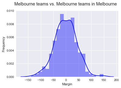
For this data (360 games), the mean is -0.825 and the median margin is -1. There is no perceptible skewness in the distribution. From this sample, it cannot be said that there is an advantage (). But is this actually important? The only differences for the home and away team in this set of games is the change rooms they use (I think?). I suspect there may be a larger ratio of home fans in attendance but given the capacity of the grounds, not many fans would be locked out. Either way it makes no perceptible difference. At least for moderate differences in crowd it’s probably acceptable to dismiss (2) as a possible predictor.

***

Let’s now consider another common gripe about Home Ground Advantage, that of the perceived favouritism of umpiring decisions. My personal view is that the free kick differential is not indicative of favouritism, and more indicative of player indiscipline. Possibly this is a mental effect from playing away from home! Without reviewing every decision and classifying each as a “justified” free kick or an “umpiring error”, it is not possible to comment on favouritism as a concept. Nevertheless, let us look at whether teams get more free kicks at home, and if this results in more wins.

This is the data from all games since 2011. In the central plot, a darker colour means a higher frequency of data. On the right-hand side is the distribution of margins (positive means a home victory) and on the top is the distribution of free kick differential (positive means more home free kicks).

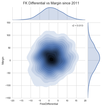
Firstly, home teams DO get more free kicks (). From the 1554 samples, on average, home sides get 1.70 more free kicks. And of course, home teams score more than their opposition, (), 7.97 points on average.

On the face of it you could easily make the connection that free kick differential correlates with the margin. The central plot tells the story that this is simply not true. The free kick differential is not a good predictor of the margin. There are many games where the free kick differential and margin have the opposite sign, almost as many as where they have the same sign. Just beacuse I’m playing around with visualisations at the moment, here is a plot of the Inside 50s differential vs. the Margin:

This is a much better predictor.

I aim to look at some of the other predictors (4-7) in a later piece after I have done some more work on it. For the moment I’m just going to consider some thoughts on how to proceed after doing this work!

***

The Scale of the Problem

There are a number of challenges facing this analysis. Firstly, let us assume the following model for predicting the outcome of a match

The team performance and player performance of each team may be predicted using their form. Environment factors include things such as HGA, the weather, and other possible factors such as if a team is coming off a short break or the bye.

To get a good measure for HGA one would need to dial out, for each past game, the effect of team performance, player performance, and non-HGA environment factors to work out an adjusted “game HGA”. From this measure, a model with each of the relevant HGA “predictors” identified could be matched.

Without doing any of the quantitative measurements, it’s easy to argue why this is going to at least be very difficult. The HGA is prevalent in the team and player performance too. Although this can be predicted from past data, this means that the full effect of HGA will be difficult to sum up. Furthermore, after removing player and team performance bias, the question remains on how to account for other environmental factors. It will likely be necessary to fit all environmental predictors (HGA, weather, etc.) simultaneously.

Then there are other problems. Is it possible that each venue has its own HGA independent of other factors? Does this change over time, i.e. how does stadium development affect this?

While I have a decent grasp on team and player performance, my model currently neglects to take weather into account (more on this in a future post I hope) and already includes HGA bias for the team and player performance. I am not in a position to attempt this quantitatively at this stage.

Nevertheless, I have some better ideas of how to proceed with this difficult problem. Firstly, I need to use player and team performance to quantify a residual “environmental” margin for each game (encompassing HGA, weather effects and noise), then examine the effects of venue, travel time, days between matches, and determine a way of describing the effect of weather.

It’s easy to see why a simple measure of HGA is attractive.

To be continued.

-Adam

 

How do you measure a player’s form?

A key part of my model is the concept that the selected players, along with the less player-specific team performance, determine the strength of the team as a whole. Here I’m going to discuss some ways to measure a player’s form to, hopefully, accurately predict their performance in an upcoming game.

Imagine for a moment each player’s value is described by a single score; I’ll use Supercoach points for this example. How do you best predict what the player’s score will be in their next game?

Speaking of Supercoach, the site provides projected scores for upcoming matches:

“Projected scores are calculated using the Herald Sun SuperCoach AFL’s proprietary formula, which takes into account several factors including the player’s most recent performances, their direct performances against the opponent and their past performance at the venue.”

This is fairly self explanatory, it uses recent form (rolling mean from n matches), form against the opposition team and form at the game’s venue. I understand the thinking behind the latter two measures but personally I would be hesitant to use them. Most players play each team only once per year; the carryover form seems tenuous unless they happen to play on the same opponent player, against the same gameplan. Likewise, the venue form will only be useful for the home team.

The AFL Ratings system uses a long-term forecast to rate a player’s value:

“A player’s rating is determined by aggregating his points tally based on a rolling window of the previous two seasons. … only a player’s most recent 40 matches are used in the calculation of his rating. … A player’s most recent 30 matches are given greater weight in determining his rating. Matches 31 through 40 are progressively reduced in weighting”

This is a different kettle of fish. The trend over a long time is a better measure of a career value, rather than a form. As I write this, Scott Pendlebury is the 5th highest rated player in the league. He’s not in good form though (**see below), so he’s unlikely to rank that highly in his next round.

How can you handle cases like Tom McDonald and James Sicily, who have been moved to the other end of the ground and their output has changed (improved?) dramatically? I think there needs to be an element of long-term and short-term form. Let’s look at some case studies using my terrible visualisations.

Here are Scott Pendlebury’s Supercoach scores for the last few years.

The first two plots have rolling means of the last 5 and 20 games respectively (**he’s clearly out of form on this measure). The final plot I’ve separated his home and away games and plotted a rolling mean of his last 10 home/away games. Maybe his calf injury is hanging around and he’s not travelling well? Let’s check some others out.

Shannon Hurn is a nicer player to model; plenty of variation as you’d expect but a nice clean upward drift on the 20-game average; it’s probably a better predictor of future performance. Lately he’s been showing better form away than at home. Bodes well for the finals.

Finally, James Sicily has gone through that transformation from forward to back and has shown a dramatic improvement in this measure. His 20-game average is taking a while to catch up and it’s likely his 5-game average will be a better predictor.

With just a few examples it’s easy to see why there are benefits with a short-term and a long-term mean. There is possibly some benefit of considering home and away form separately too.

My model considers a weight of these three means for predicting the mean output of a player – their current form. Each of the seven (!) parameters I use to measure a player’s performance gets a mean of this form. The choice of 5- and 20-game means passes the eye test (for me, anyway) and gives good outcomes when simulating past seasons. Rookie players with n<5 games just have a mean of all of their performances, players with 5<n<20 get a 5-game mean and a n-game mean.

***

Now, what about the game-to-game variance from the mean(s)? The means will be good for giving a mean outcomes but variance will be useful in determining the probability of outcomes. In the finance industry, estimating volatility is where the money is.

I need to do more investigation on the best way of handling this, and I might write a piece when it’s a little more refined. My current method is to take a sample standard deviation of the measure over 10 games. I had been using 5 games and this was giving me some strange outcomes. Having done some more simulations, 10 seems to work pretty well as compared to larger and smaller samples.

Cheers for now!

-Adam